Is This Drawdown Evidence, Or Just Noise?

You are 600 bets into a profitable strategy. Your equity curve reached a new peak three weeks ago and has been falling ever since. You are now 55 units below that peak.

The question is not whether your strategy was ever good. It is whether this drawdown is consistent with the strategy still being good.

There is a precise way to answer it.

The Parameters Your Model Gives You

Assume you bet a flat stake at decimal odds $O$, and your model estimates a true win probability of $p$. As in previous articles, the expected profit per bet is:

$$\mu = pO - 1$$

And the variance per bet is:

$$\sigma^2 = p(1-p)O^2$$

For a $5\%$ edge at three different odds levels:

Odds	Win probability	σ²	σ²/μ
1.5	0.700	0.47	9.4 units
3.0	0.350	2.05	40.9 units
8.0	0.131	7.30	145.9 units

The ratio $\sigma^2 / \mu$ is the natural scale for drawdowns in each strategy. At identical edge, long odds carry more than fifteen times the drawdown risk of short odds. The next section shows what this looks like in practice.

Simulating What Your Model Predicts

A Monte Carlo simulation generates thousands of synthetic equity curves using the model's parameters. For each simulated bettor, we record the maximum drawdown: the largest peak-to-trough decline over the full sample.

The result is the null distribution for your drawdown. It shows what outcomes are consistent with the model, and which are unusual.

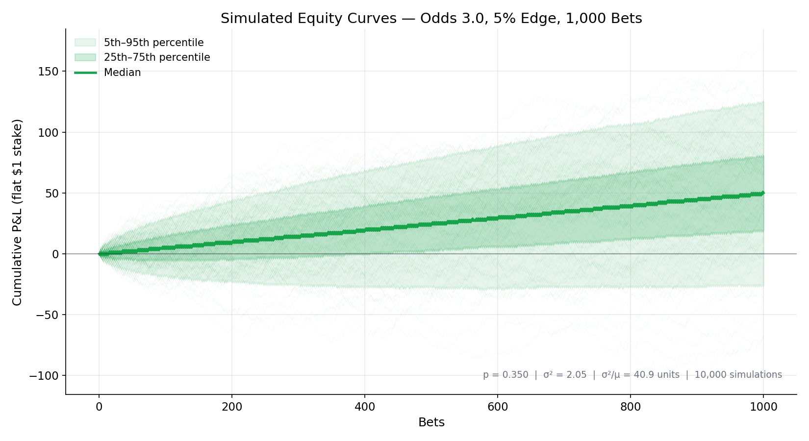
The shaded bands show the 5th–95th and 25th–75th percentile ranges across 10,000 simulations. The spread is large. A correctly-specified model produces a very wide range of outcomes over 1,000 bets.

Running the same simulation for each odds level and recording the maximum drawdown from each path gives the distributions below.

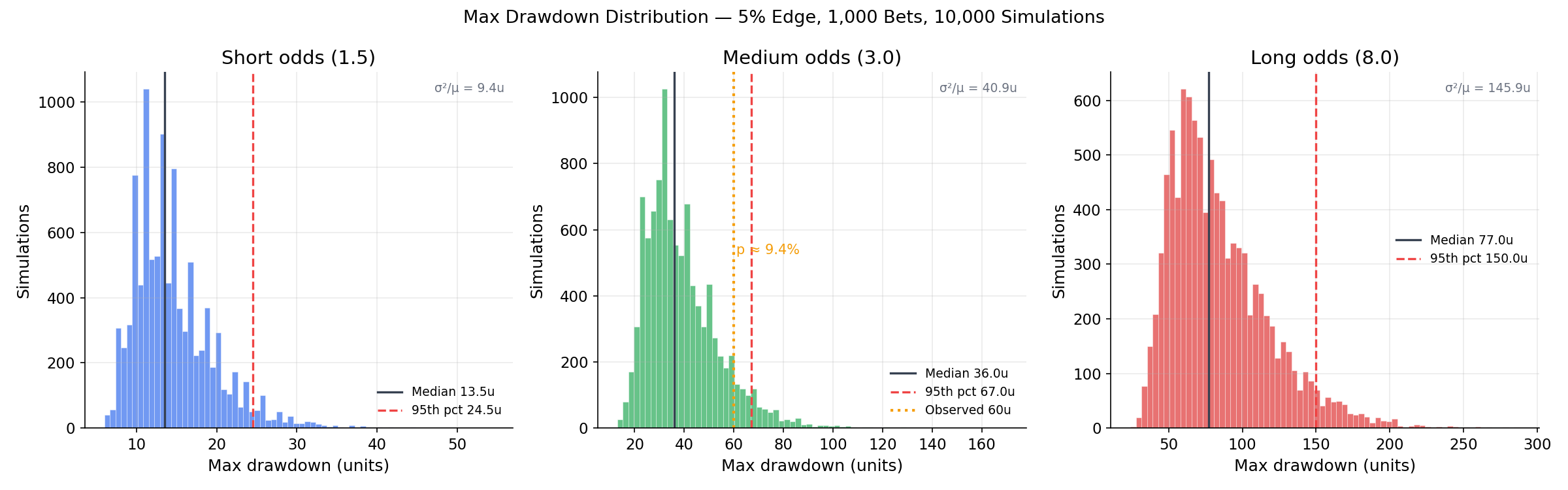
The difference is striking. At odds $1.5$, the median max drawdown is around 13 units. At odds $3.0$, it is 36 units. At odds $8.0$, it is 77 units. All three strategies have the same $5\%$ edge. Only the variance differs.

Reading A P-Value From The Simulation

The middle panel illustrates how to apply this in practice. Suppose a strategy at odds $3.0$ is showing a current max drawdown of $60$ units. The dotted orange line marks this value.

The area to the right of that line — the fraction of simulations with a max drawdown of $60$ units or more — is the p-value. In this case, around $9.4\%$ of correctly-modelled strategies over 1,000 bets produce a drawdown this large.

Formally:

$$p = P(\text{MDD}_N \geq d \mid \text{model correct})$$

A p-value of $9.4\%$ says: if the strategy is working exactly as modelled, roughly one in ten simulated bettors would have experienced at least this drawdown after 1,000 bets. Uncomfortable, but within the expected range.

If the same 60-unit drawdown appeared in a strategy at odds $1.5$, the p-value would be far below $1\%$. At short odds, a 60-unit drawdown is not just unlucky — it is nearly impossible under a working model with $5\%$ edge.

The Analytical Formula

There is a clean result from Brownian motion theory that gives intuition about the scale of drawdowns without simulation.

For a strategy with drift $\mu$ and per-bet variance $\sigma^2$, the drawdown process — the distance below the running peak at any given moment — converges in the long run to an exponential distribution with mean $\sigma^2 / (2\mu)$.

This means the probability that the current drawdown from the most recent peak exceeds $d$ is approximately:

$$P(D > d) \approx e^{-2\mu d / \sigma^2}$$

Each time the equity curve sets a new maximum, a fresh excursion begins. The probability that excursion falls at least $d$ below the new peak — before the next new maximum is reached — is $e^{-2\mu d / \sigma^2}$.

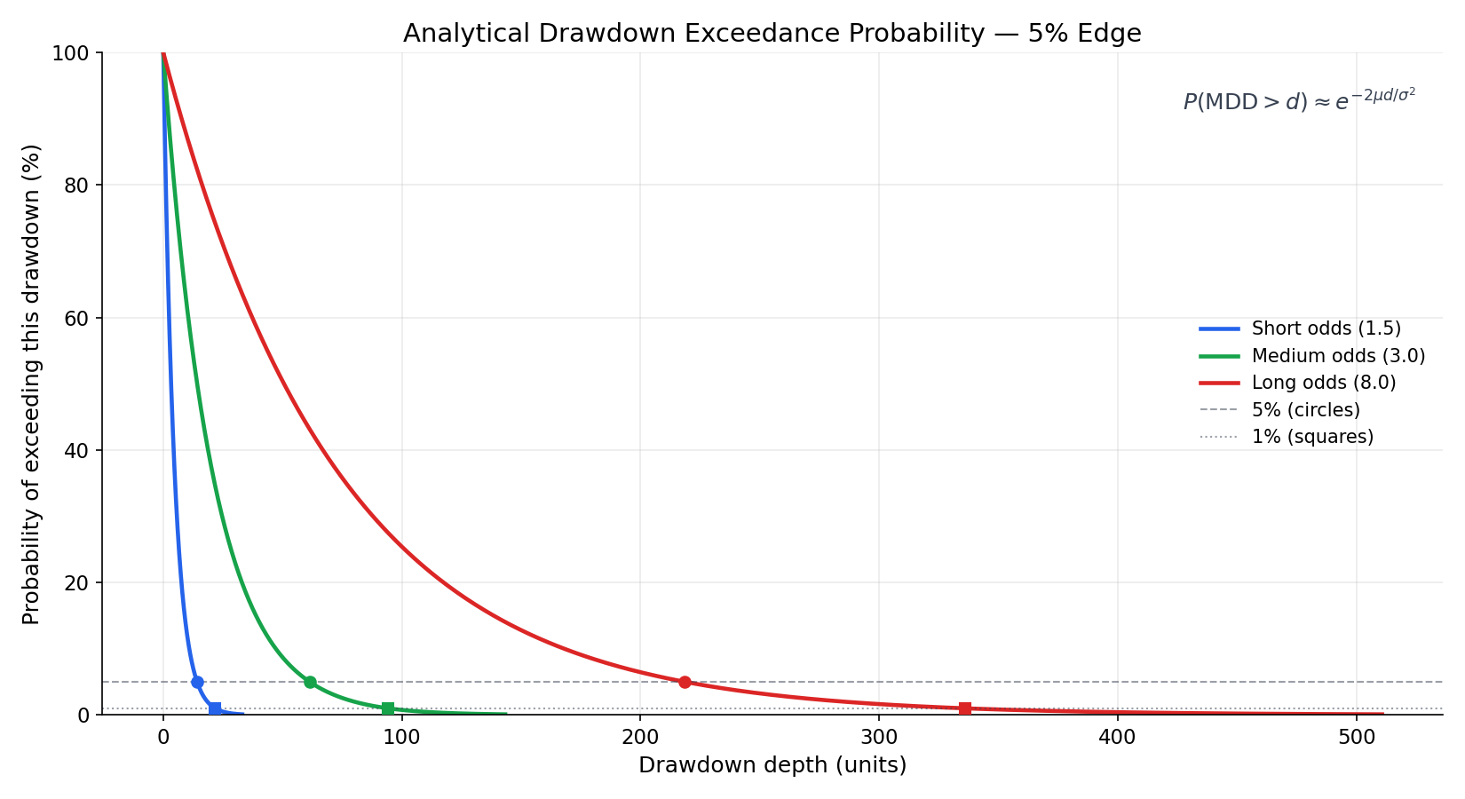
The three curves show the same $5\%$ edge at different odds. The circles mark the point where the probability drops to $5\%$. The squares mark $1\%$.

Odds	Depth where P = 5%	Depth where P = 1%
1.5	14 units	22 units
3.0	61 units	94 units
8.0	219 units	337 units

These numbers should recalibrate what counts as alarming. A strategy at odds $8.0$ with $5\%$ edge should regularly produce drawdowns in the double digits from any given peak. A 100-unit drawdown from the current high is expected roughly $25\%$ of the time:

$$e^{-2 \times 0.05 \times 100 / 7.30} \approx 25\%$$

For a short-odds strategy, the same 100-unit drawdown would be essentially impossible.

The Natural Scale

The formula makes the key ratio explicit. Setting $P = 5\%$ and solving for $d$:

$$d_{5\%} = \frac{\sigma^2}{2\mu} \ln 20 \approx 1.5 \cdot \frac{\sigma^2}{\mu}$$

The quantity $\sigma^2 / \mu$ is the only scale that matters. Drawdowns much smaller than this are routine. Drawdowns many times this scale are evidence that something has changed.

Two strategies can have the same edge and opposite risk profiles purely because of their odds. A bettor who moves from short odds to long odds without adjusting their expectations for drawdown will be constantly mistaking normal variance for model failure.

Upswings Are Symmetric

The same logic applies to unexpectedly good runs.

If the equity curve is sitting in the 95th percentile of the simulation distribution, that is also an extreme outcome. The model may be too conservative. The sample period may have been unusually favourable. Or it may simply be variance.

The simulation gives the null distribution in both directions. A result in the top $5\%$ upswing is equivalent evidence that something is different from what the model predicts, just in the opposite direction.

Practical Interpretation

The p-value from the simulation is continuous evidence, not a pass or fail.

• $p > 10\%$: routine variance, no signal
• $p \in [5\%, 10\%]$: mildly unusual, worth noting
• $p \in [1\%, 5\%]$: meaningful signal — review whether the model's parameters still hold
• $p < 1\%$: strong evidence that something has changed

A drawdown in the bottom $5\%$ of the simulated distribution means that if you ran the same strategy from scratch 100 times, only five would have produced a drawdown this bad. That is meaningful information without requiring formal hypothesis testing.

Putting It Together

Simulating the null distribution takes a few lines of code. For a given $p$, $O$, and $N$:

1. Simulate $10{,}000$ equity curves: each bet is a win with probability $p$ and a loss otherwise.
2. For each curve, compute the max drawdown.
3. Find what fraction of max drawdowns exceed your observed value. That fraction is your p-value.

The analytical formula provides a quick sanity check and a way to reason about scale without simulation. For precise probabilities over a specific number of bets, the simulation is more accurate.

The uncomfortable truth for long-odds bettors is that drawdowns which look catastrophic are often statistically unremarkable. The goal is not to have no drawdowns. The goal is to have drawdowns that are consistent with the model. When they are, you have no additional reason to stop. When they are not, you have a testable signal that something has changed — and the mathematics to distinguish between the two.